Getting Started
A distance function(also referred as a metric) in mathematics refers to the function that defines a distance between any two points of a set. The most prevalent example is the Euclidean distance. But let’s first define what makes a function a distance function.
For a function to be a distance function, it has to satisfy the following properties$^{[1]}$
:
- Non-negativity :
$d(x, y) \geq 0$ - Identity :
$d(x, y) = 0 \iff x=y$ - Symmetry :
$d(x, y) = d(y, x)$ - Triangle Inequality :
$d(x, z) \leq d(x, y) + d(y, z)$
Some of the distance functions which we went over in class were $L_p$ distances, Jaccard Distance, Cosine Distance and Edit distance. Now let’s take a look at one another kind of distance and then let’s take a look at what happens to distances in high dimensional spaces.
I: Kullback–Leibler divergence
KL divergence is used to measure the difference between two probability distributions over the same random variable x.
$$D_{KL}(p(x)||q(x)) = \sum_{x \in X} p(x) \ln \frac{p(x)}{q(x)}$$
In terms of information theory, KL divergence measures the expected number of extra bits required to code samples from distribution $p(x)$ when using code based on $q(x)$. Another way to think about this is that $p(x)$ is the true distribution of data and $q(x)$ is our approximation of it. $^{[2]}$
Even though it looks like KL divergence measures distance between two probability distributions, it is not a distance measure. KL divergence is neither symmetric not does it satisfy the triangle inequality. It is however non-negative.
If it is not a distance metric, then how is it used? In the formula presented above, the true distribution is often intractable. Therefore by minimizing the KL divergence by using tractable approximated distributions we can get an approximate distribution from which samples can be drawn.
Here’s another interesting property. Maximum Likelihood Estimation is one of the ways of estimating the parameters of a model. It attempts to find the parameters which maximize the likelihood function. Utilizing MLE for logistic regression is a common application.
However the interesting part is the fact that maximizing the likelihood is equivalent to minimizing $$D_{KL}(P(x|\theta^*)||P(X|\theta))$$
where $P(.|\theta^*)$ is the true distribution and $P(.|\theta)$ is our estimate of it. Let’s see how
$$D_{KL}(P(x|\theta^*)||P(x|\theta))=\sum_{x \in X} P(x|\theta^*) \ln \frac{P(x|\theta^*)}{P(x|\theta)}$$
$$=\sum_{x \in X} [P(x|\theta^*) \ln P(x|\theta^*) - P(x|\theta^*) \ln P(x|\theta)]$$
The first term is nothing but the entropy of $P(x|\theta^*)$
$$= -H[P(x|\theta^*)] - \sum_{x \in X} P(x|\theta^*) \ln P(x|\theta)$$
Since the first term has nothing to do with the parameters represented by $\theta$, therefore we can drop it. Therefore
$$D_{KL}(P(x|\theta^*)||P(X|\theta)) \propto - \sum_{x \in X}P(x|\theta^*) \ln P(x|\theta)$$
Now if we draw N samples $x ~ P(x|\theta^*)$
$$D_{KL}(P(x|\theta^*)||P(X|\theta)) \propto - \sum_{x \in X} [\frac{1}{N}\sum_{i=1}^N \delta(x-x_i)]\ln P(x|\theta)$$
By the law of large numbers as N approaches infinity, the above equation can be written as
$$D_{KL}(P(x|\theta^*)||P(X|\theta)) \propto - \frac{1}{N}\sum_{i=1}^N \ln P(x_i|\theta)$$
which is nothing but the log likelihood of the data. This is specially important as it shows us that maximizing the likelihood of data using our estimate is equivalent to minimizing the difference between the true distribution and our estimate. Hence even if the true distribution is unknown, MLE can be used as a tool to apply our estimate to the true distribution.
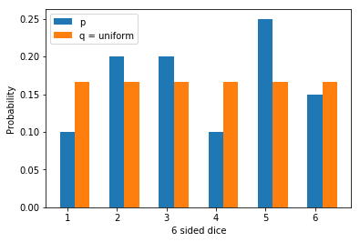
Before we finish our discussion of KL divergence let’s see a toy example. Assuming that we have a 6 sided weighted dice such that the true probabilities are given by $$p=[0.1, 0.2, 0.2, 0.1, 0.25, 0.15]$$. If we try to model it using a uniform distribution, our $q$ becomes $$q=[0.166, 0.166, 0.166, 0.166, 0.166, 0.166]$$.
The figure below shows the bar plot for the same
We can write a simple code snippet which can help us calculate the KL divergence between two distributions.(Disclaimer: For a much robust implementation refer to the scipy package)
import numpy as np

def kl_div(p, q):
    p = np.asarray(p, dtype=np.float)
    q = np.asarray(q, dtype=np.float)

    return np.sum(np.where(p!=0, p*np.log(p/q), 0))
Using our toy example,
>>print(kl_div(p, q))
0.0603337190402897
>>print(kl_div(q, p))
0.055253998576011196
This non symmetric nature of KL divergence as discussed above is one of the reasons it is not a distance metric.
II: Curse of Dimensionality
A typical supervised machine learning problem involves examples which are essentially vectors in a high dimensional feature space. A feature vector $x=<x_1, x_2, x_3, ..., x_d>$, can be said to be belonging to the space $\mathbb{R}^D$
Recall the concepts underlying K-Nearest Neighbors. We utilize the labels of the K nearest points to make prediction about the label of the point under consideration. This is done because of our inductive bias that if a point lies in a space, then it is similar to other points which are in vicinity to it. Each dimension of the feature vector is taken into consideration when the concept of nearest is being applied. However this introduces a couple of problems. Since KNN is giving importance to all features equally, in a dataset containing only a select relevant features KNN can perform poorly.
Another problem which arises is of feature scaling. Let’s assume that the distance metric for KNN is Euclidean distance. In such a case different scales amongst the dimensions of the feature vector can result in some dimensions being completely ignored. However, this has an easy fix. We can scale the dimensions to zero mean and unit variance and get rid of this issue.
However, the problem becomes much more severe when the number of dimensions start increasing.
Extending from the analysis for KNN explained above, let us try to consider a nearest-neighbor estimate of a point at the origin on a p dimensional space. Consider that there are N points that are uniformly distributed in this p dimensional unit ball around the point at center. Given this situation, let us try to compute the median distance of the closest data point to the center.
The volume in the space more than a distance $kr$ from the center where $r$ is the radius of the ball, is proportional to $$\frac{r^{p} - (kr)^{p}}{r^{p}} = 1 - k^{p}$$
Probability that N points are at a distance greater than $kr$ is $(1 - k^{p})^{N}$ $^{[3]}$. So, to get the median distance of nearest point from center, set this probability to 0.5
$$(1 - k^{p})^{N} = \frac{1}{2}$$
$$\implies k = (1 - \frac{1}{2}^{\frac{1}{N}})^\frac{1}{p} $$
This says that for a fixed number of data points, as the number of dimensions increase, the samples tend to aggregate near the boundary of the sample space which makes it difficult for the model to predict near the boundaries.
This can be corroborated by the following experiment, where 1000 points of p dimensions are generated where on each dimension, the value is uniformly distributed between [0,1] and all of the dimensions are independent. The distribution of distances between the points look as follows.
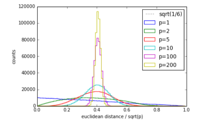
We can see that the distances have become more concentrated as p increases from what we expected above and gives us the idea that it becomes more and more difficult to cluster points based on mere distance. Even though real data wouldn’t have independent and uniformly distributed dimensions, the probability that different points have similar distances is definitely higher.